Additive manufacturing in 2024 can be done through multiple different processes. In this blog post, we will be focusing on the process of FMD/FFM printing. FDM/FFM uses a roll of filament as the material that is extruded through a hot end of a printer to make lines that can build upon each other. This post will go over the process of making a custom 3D printing slicer and then comparing it to a commercially available slicer (Prusa Slicer). The main goal of this post is to demonstrate all the difficulties of creating a FDM/FFM slicer that are not often thought of when using them.
Task 1: Making the Slicer
Before anything can be printed, a slicer must be implemented and tested to be sure the printer will not break. As always, the code can be found on my GitHub, this time under the name “L3-3DPSlicerGcodeGenerator1.gh”.
Part 1: Generating the Slices
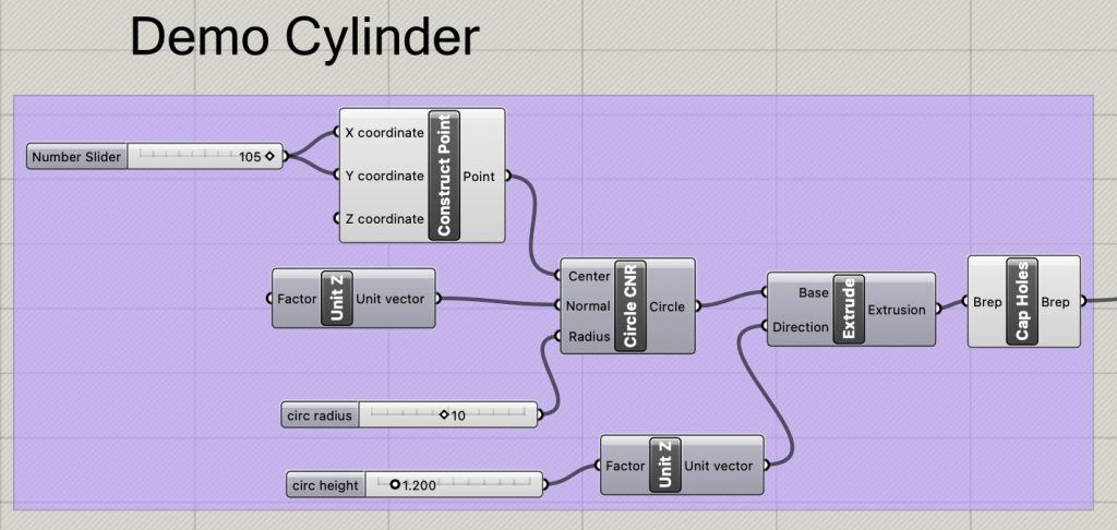
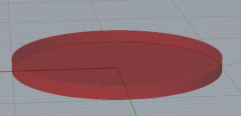
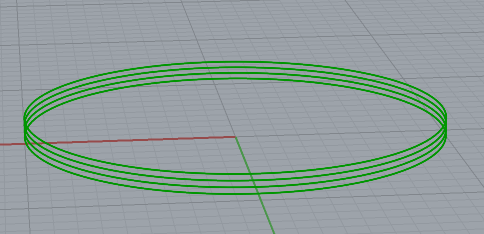
For this section, a demo cylinder of 1.2mm height and 10mm radius will be used. This cylinder will show the process of how the slicer approaches breaking up an object and then generating the layer and infill lines.
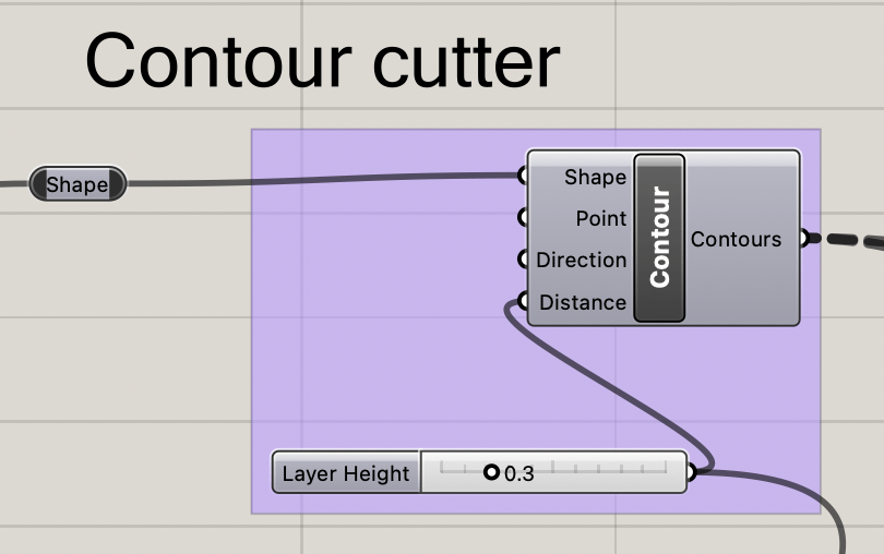
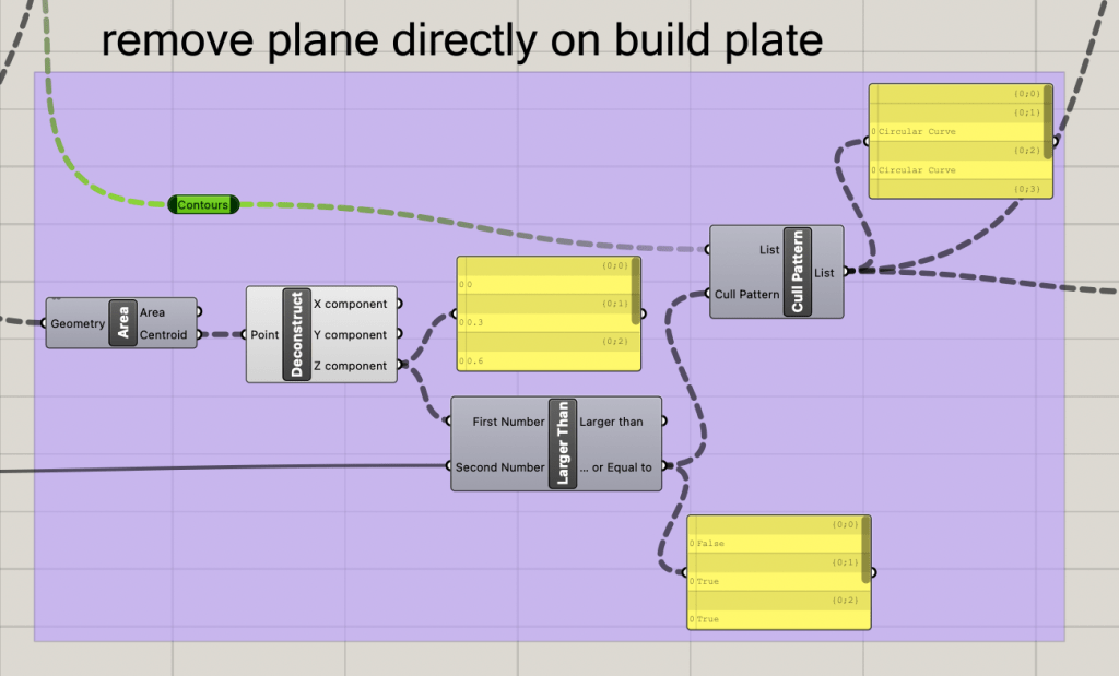
The first act is splitting the outside of the cylinder into independent curves using the contour node. The contour node requires a specified distance between each item, and the provided layer hight of 0.3mm is the desired value. Note that the current contour shapes includes an outline at Z = 0, this cannot be printed, so we will have to filter out all values that would be below the printer’s build plate.
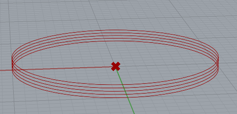
Using the output of the contours, we create a list and compare the Z component of each item in the list to see if any are less that 1 layer height. Any contours that are below this threshold will be removed from the queue by the cull pattern node.
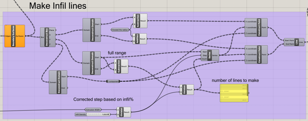
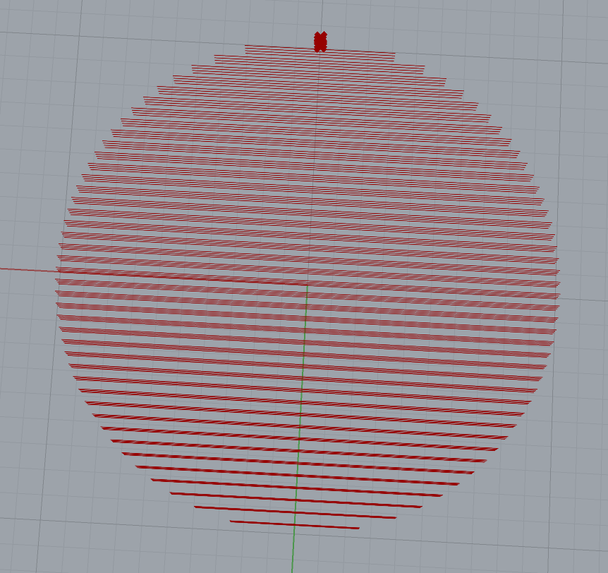
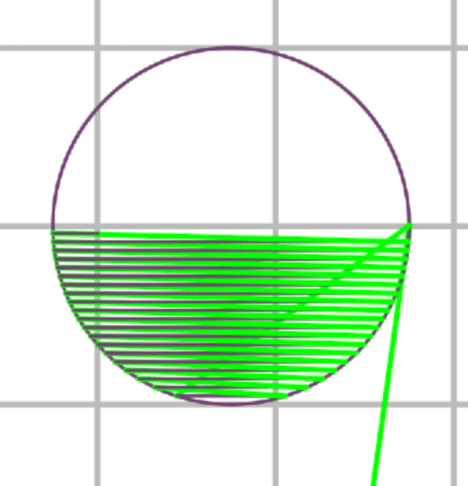
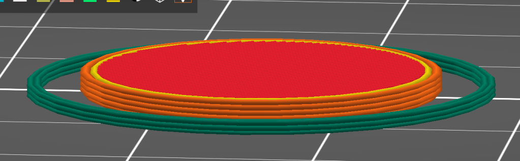
Now that we have the accepted contour curves, we can create the infill for each layer. For this blog post, the infill will be simple disconnected parallel lines. The box dimensions of each contour are used to create a rectangle of lines that will stretch slightly over the contour to encapsulate everything as an infill line. Because the demo item is a cylinder, all of the infill rectangles will be the same. Each infill line is spaced accordingly to the extrusion width that the filament expands to when released from the hot end. There is also a percentage fill amount that can further increase the spacing, by decreasing the percentage fill, the amount of infill lines decreases, while the spacing between each will increase.
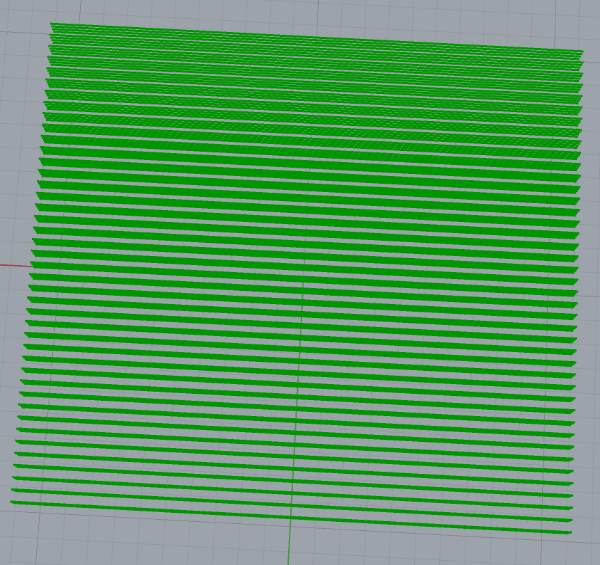
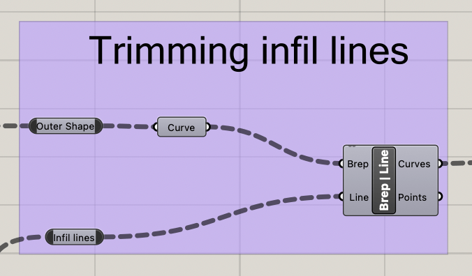
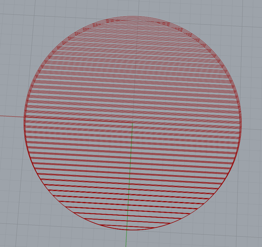
We can now trim the infill lines to fit the shape correctly with a brep line node that will use the corresponding contour to remove excess infill. The result is the trimmed infill lines, we now need to join the contour and infill lines correctly.
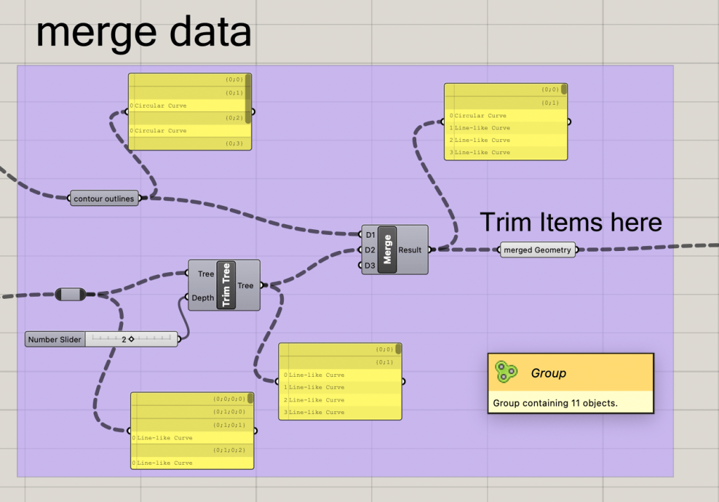
By default, the infill and contour exist on different tree levels and are incompatible when data merging. To fix this we first use a trim tree node to remove two layer of useless lists on the infill. We then merge the contour with the corresponding infill to make each layer a corresponding list. It is very important that the contour is placed above the infill on the merge node inputs, as the order determines what will be sent to the G-Code editor first.
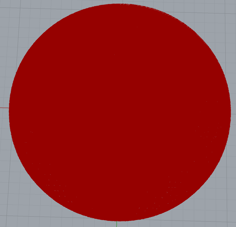
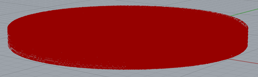
We will now remove any excess commands and then explode the geometry of each slice so that the system can turn curves into direct line commands. The individual lines cannot be seen as the end points are also being displayed and are blocking out any of the lines, so that the object looks solid once again.
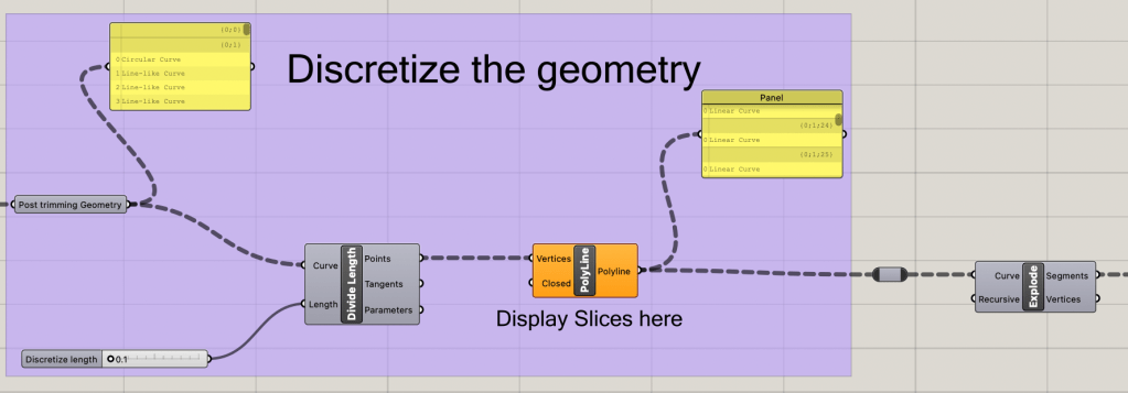
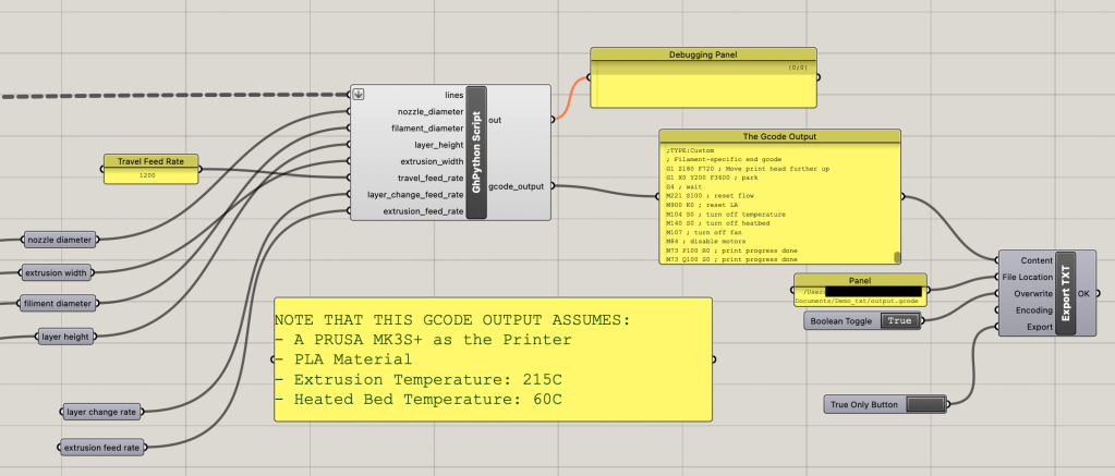
The lines are then fed into the grasshopper python script node to turn each line into a G-Code command. The act of creating the G-Code will be discussed in Part 2, along with the parameter values. After being converted, the G-Code is then placed into an export text node, from the pancake plugin for grasshopper. This text can then be sent to a designated file location to be saved. Note that the system is already expecting a G-Code file there, as the text export did not want to create something out of nothing.
Part 2: Generating the G-Code
Most of the Python code will act similarly, so an overview of the main sections will be discussed, while not covering everything. As always, check my GitHub page for the original files. Attached below is the set of values that will correspond to the expected values that a Prussia Mk3 will be using when actually printing the sliced model.
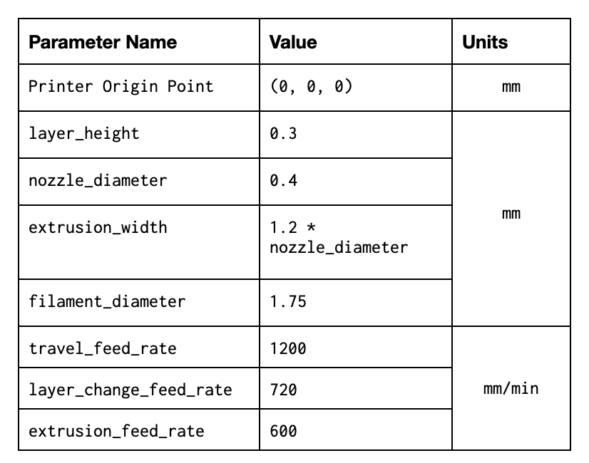
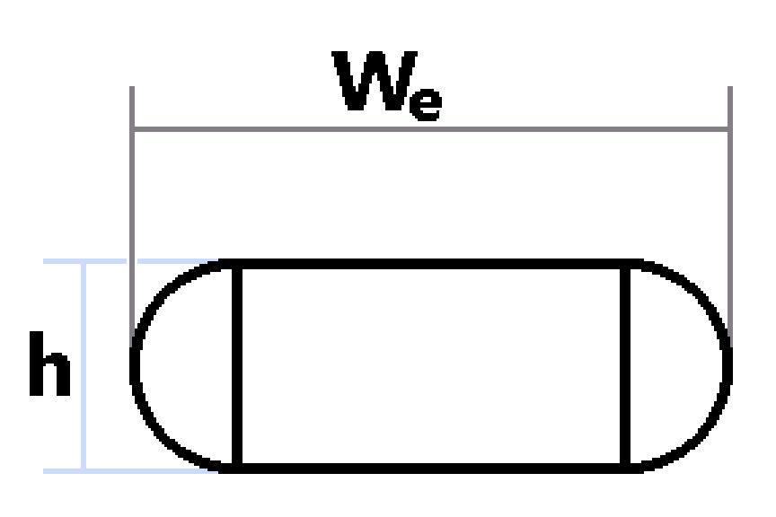
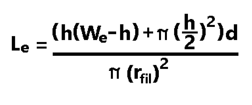
The math for the correct extrusion amount is based on the above table and the concept that the extruder will output the same amount of material as is taken in. This amount of material moved into the hot end of the printer is the “E” value of all G1 G-Code commands. Because we know the incoming volume is the distance of filament being driven in {Le}(the item we are looking for) multiplied by the area of the filament (Pi*radius^2), We can isolate Le by dividing the output volume by the area of the filament. The output volume will be the distance {d} traveled multiplied by the area of the extruded material. Below is an example of the extruded material, where We is the extrusion width and h is the layer height. Notice that the two main shapes are a rectangle, and two half circles.
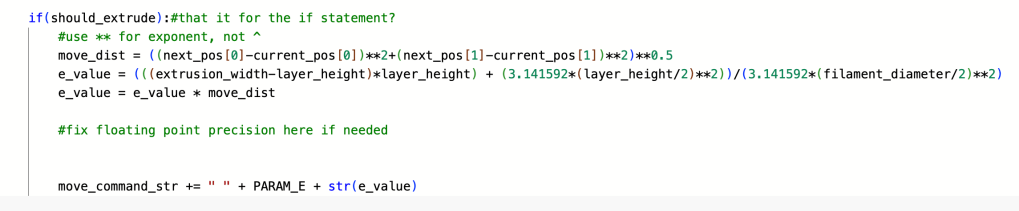
Now that we have the correct equation and the reason behind using it, we can write the part of the python code that will handle calculating the E value when we are extruding filament. We take the distance between the x and y component of the given line (We don’t use the z component because of check we will do later on so that everything is on the same level beforehand). We then calculate the value of Le according to the equation above. We can then concatenate this as part of the move_command string.
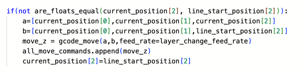
Before any planar move command is run in the system, we need to check if the z component of the starting line and where the printer head are is the same. If these values are different, we will move the printer head up to the new z position (only the z position, not moving in either x or y) and make note of that internally.
After position correcting for the x and y components, we can then start extruding, by calling the code_move command with the should_extrude value set to true, we will call the extrusion math equation show earlier and move the print head while extruding the correct amount of filament.
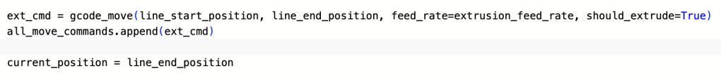
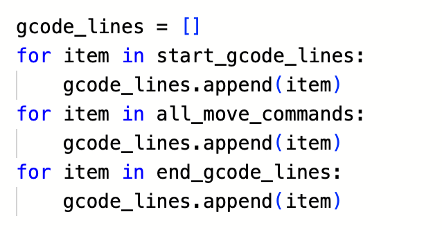
After all the lines have been turned into G-Code commands, we then merge all of the commands with the start up and ending G-Code. The order of this code matters as always, so the list is first populated with the starting code, then the line code, and finally the ending code. This text list is then output and sent into the export node to be saved as a real g-code file.
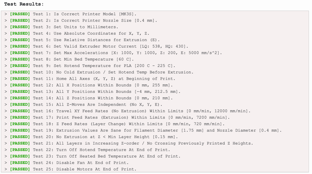
Part 3: Testing the G-Code
The testing of the G-Code was done through two main methods; Viewing the exported code through a G-Code viewer online, and through a G-Code checker make for my Computational Fabrication class. Using both of these can help with spotting any issues that may have been created that only one of these programs may not have seen.
Task 2: Printing and Slicer Comparison
Now with functioning G-Code, we can test the differences in slicers. The testing object will be a cylinder of 1.5mm height and 20mm radius. Once again, the printing was done at the BTU lab on the CU Boulder campus. With the Prusa Mk3 printer, there are a few details that can be used as a benchmark for these prints, namely the pattern on the buildplate, layer line consistency and the infill. If the print is able to display the pattern after being removed, there was great bedplate adheason.
Results of the Prusa Sliced Cylinder
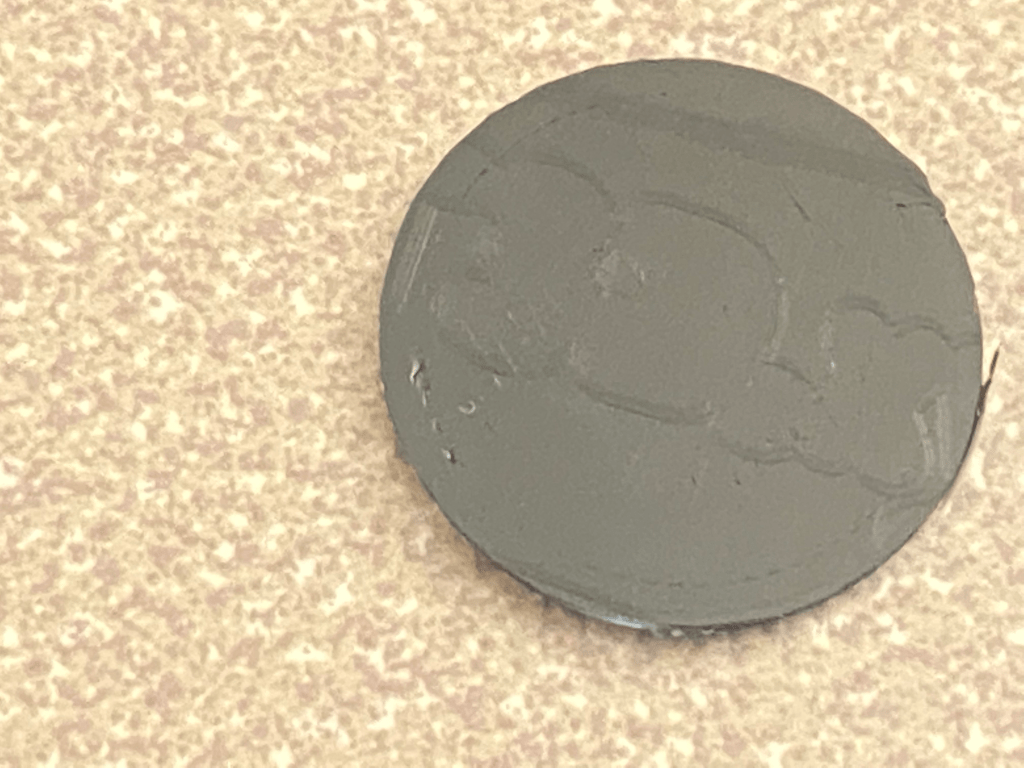
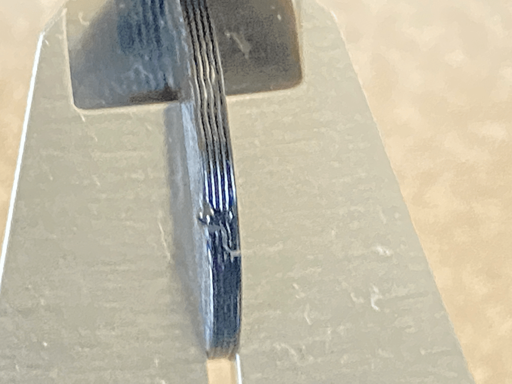
{bed adhesion, layer comparison and tracking of infill}
For the Prusa sliced cylinder, the results are as expected, very good. Due to the glare when I was trying to capture the detail of the bottom of the cylinder, the printbed pattern cannot be seen as well as it is actually implanted on the print. The bottom layer is also entirely solid, you cannot see any infill lines on the first layer, it looks homogenous. From a measure meant standpoint, the diameter measures 20.09mm with a total height of 1.36mm, the layer heigh inaccuracy is to be expected as most printers will normally force the layers slightly closer together to allow for better layer adhesion. From the provided picture of the layer lines, five distinct layers can be see, where the first and second are much closer compared to the remaining layers. The top layer infill is seemingly vertical lines with no direct connection, but this is overlooking infill optomiatins done when slicing.

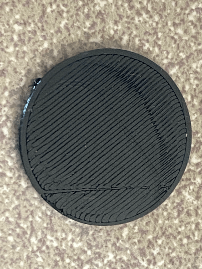
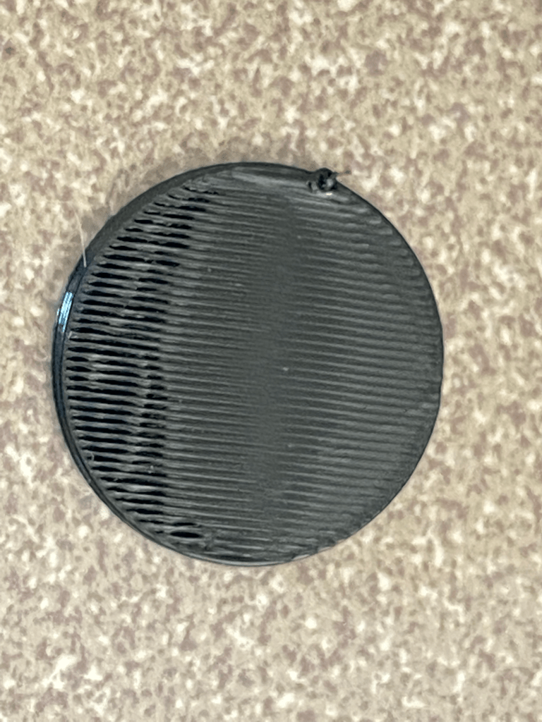
Results of the Custom Sliced Cylinder
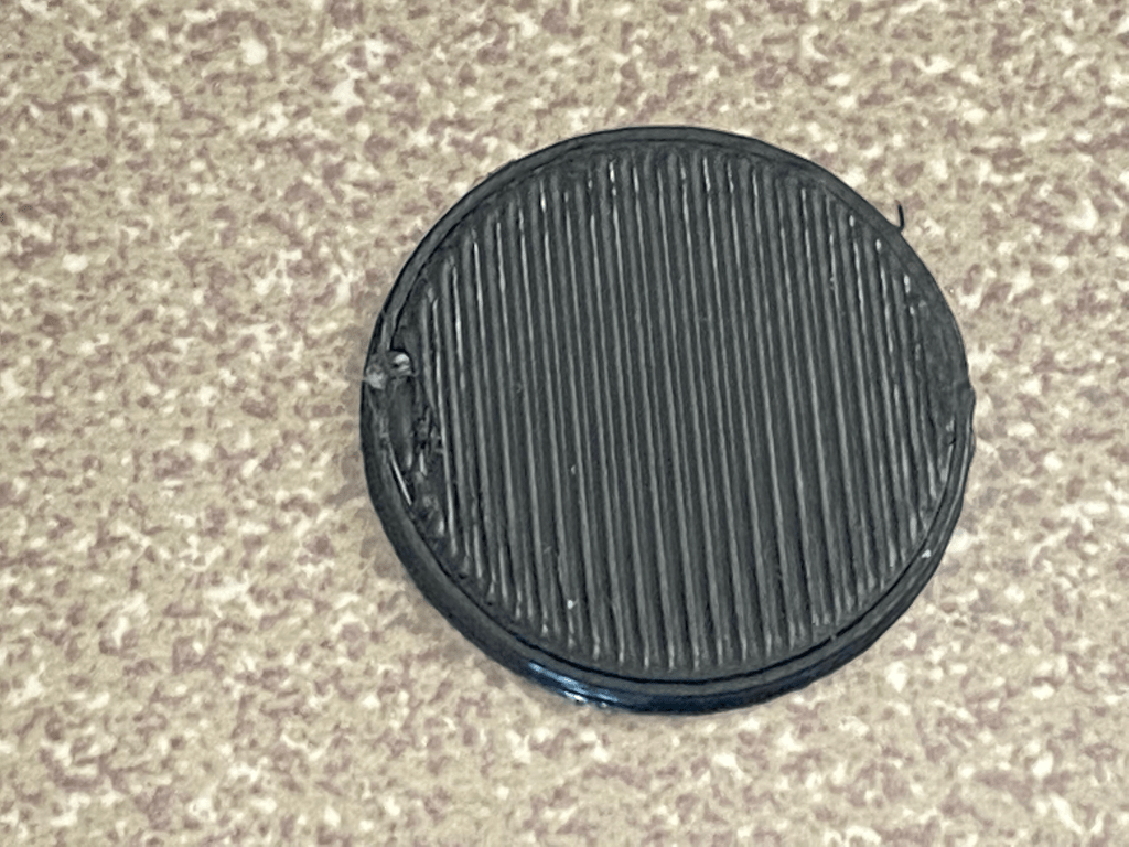
With the custom sliced cylinder, the results are better than I was expecting. Though the first layer, isn’t fully joined like the Prusa slicer cylinder, some of the printbed pattern can be seen, though not in the picture provided. From a measurement standpoint this cylinder is bigger. With a diameter of 20.44mm and a layerheight of 1.59mm, this print over acceeds the given dimensions of the cylinder STL file. The top infill layer is slightly pattchy, the miscoloration in the third image is not shading, but gaps in the infill. My best guess is that as the nozzle moves across to restart the next infill command, some of the plastic residue is being placed into the created crevices and is helping with the infill. Thi sleaves about two thirds with the correct amount of infil and the last third missing half of the needed infill.
One major aspect of the printing process is the time spend printing, when comparing those values the Prusa sliced cylinder took half as long. This time discrepancy can be chalked up to multiple sources, but the major culprit is the infill method. The custom infill method requires the print head to travel across the print after each infill line without using more material, this leads to double the moves thus increasing the print time.
Conclusion
Slicers are able to do multiple things under the hood that the user will never really notice. Creating an efficient infill patten is a work of mathematic harmony as to not waste both time and material, while providing support and stability. The infill pattern created in this post wastes time a large amount of time with unoptimized travel, as it will make a line and then travel back to the other side of the shape to go in the same direction again. This motion wastes time and could lead to stringing in the print if the infill amount wasn’t 100%.

Leave a comment